In machine learning, the inclusion of the most predictive features in an algorithm typically yields superior results. For my Master’s thesis, I was tasked with the creation of a prediction engine for invoice payments, an engine that attempts to predict the payment dates of newly issued invoices.
As someone with prior experience predicting invoice payments, I knew past payment behavior could provide a fairly accurate forecast of future payments. This understanding was reinforced by the literature I reviewed, which highlighted various customer and global arrears windows as predictive indicators within this context. Now that I knew what I wanted, I needed a method to execute it in Python. This is where I discovered the rolling function. If you prefer a more visual approach, you can watch the accompanying YouTube video instead of following the method outlined in the text below.
The code for the following example, along with the dataset used, can be accessed on GitHub through this link
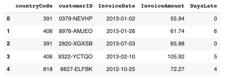
The dataset used in this example comprises 2466 invoices spanning a period of approximately two years. The objective is to construct four window functions that examine past invoices at the customer and global levels, both for a quantity-based window of three invoices and a time-based window of 30 days. After importing pandas and cleaning the data to only include the columns relevant to this example, we are left with the following snapshot of the dataset.

The creation of global functions is quite straightforward, as illustrated by the code below. It is imperative to convert the date to a datetime format and sort it before proceeding. With that completed, we create a new column in the dataset and set it as ‘df’. This is achieved through the command df.rolling(window = ‘30d’, on= “InvoiceDate”).DaysLate.mean(). What this function does is take the 30 days prior to the invoice (by Invoice Date) and calculate the average of the ‘DaysLate’ column.
df["InvoiceDate"] = pd.to_datetime(df["InvoiceDate"])
df = df.sort_values('InvoiceDate')
# Global Days Late Last 30 Days
df["GlobalDaysLateLast30days"] = df.rolling(window = '30d', on = "InvoiceDate").DaysLate.mean()
Creating quantity-based window aggregates is just as straightforward. The only difference is the substitution of a day aggregate with a whole number. This adjustment will yield the average of the last three invoices. To avoid NaN values in this scenario, you can set the ‘min_periods’ parameter to 1. This will provide an average even if the algorithm has fewer than three records at its disposal.# Global Days Late Last 3 Invoices (min_periods = 1 to avoid NaN)
df["GlobalDaysLateLast3Inv"] = df.rolling(window = 3, on = "InvoiceDate")
.DaysLate.mean()
Below, you can see the output produced by these functions. We could have circumvented the NaN values by setting ‘min_periods’ to 1, which is exactly what we’ll be doing at the customer level.

We adhere to the same approach at the customer level, but the code becomes slightly more intricate. This is primarily due to the requirement for implementing groupings and adjusting the indices. Below, you’ll find the code snippet that enables us to calculate the average of the three most recent invoices at the customer level.
# Customer last 3 Invoices average days late
df["AvLateLast3"] = df.groupby("customerID")
.rolling(window = 3,min_periods = 1)
.DaysLate.mean().reset_index().set_index("level_1")
.sort_index()["DaysLate"]
The time-based grouping further complicates the process as we first need to generate the data point before merging it back into the dataframe. You can find the corresponding code for this operation below.
# Customer Average Days Late Last 30 days
mean_30d = (df .set_index('InvoiceDate') # !important
.sort_index() .groupby('customerID')
.rolling('30d')['DaysLate']
.mean()
.reset_index(name='CustomerDaysLate_30days') )
# merge the rolling mean back to original dataframe
df = df.merge(mean_30d)
As you can see in the final dataset, we have successfully executed window functions at both the global and customer levels. The example for one customer is below.

I have found these methods to be incredibly valuable in crafting features for machine learning. I’m genuinely interested to hear about your experiences implementing them or any suggestions you might have for enhancing the code provided above. Please feel free to share your thoughts in the comments section. Happy coding!